Introduction to the BGV encryption scheme

Scope
This is the 2nd article of our blog series on Fully Homomorphic Encryption (FHE) and its applications. In the previous article, we introduce the readers to the levelled Brakerski/Fan-Vercauteren scheme [Bra12, FV12]. Here, we will describe the levelled Brakerski-Gentry-Vaikuntanathan (BGV) [BGV14] scheme, another Ring-Learning with Errors (RLWE)-based cryptosystem that offers computing on encrypted data. BGV and BFV offer the same capability, i.e., exact computation on integral messages, however, they have a few differences in their construction that will become evident in this article. Note: this article is also available as a PDF Document .

The BGV scheme is another FHE scheme that belongs to the second generation of FHE schemes. Its security stems from the hardness of the Ring-Learning with Errors (RLWE) problem [LPR13].

Similar to the BFV scheme, BGV defines plaintext and ciphertext rings. The encryption procedure maps input plaintext elements of the plaintext ring to ciphertext elements of the ciphertext ring. Broadly speaking, encryption is done by concealing the plaintext message with an almost random mask that is computed using the public key (or the secret key in the symmetric-key operation mode). The output of encryption is typically two elements of the ciphertext space; the first of which contains the masked plaintext data whereas the second contains auxiliary information that can be used in the decryption procedure. Decryption uses the secret key and the auxiliary information in the ciphertext to remove the mask and recover the plaintext message. This might ring a bell for the readers who are familiar with ElGamal encryption [ElG21] which maps a single plaintext element to a paired-element ciphertext.

One crucial notion in RLWE-based FHE schemes is the error, also known as noise, that is added to the plaintext message during encryption. The error is crucial to satisfy the RLWE hardness assumptions, or else the RLWE would turn into an easy computational problem that can be solved by commodity computing machines and as a result, it would render FHE schemes built on such easy problems easy to break. Recall that in BFV, the error magnitude grows as we perform homomorphic evaluations (mainly, homomorphic addition and homomorphic multiplication). BGV exhibits similar noise behaviour, i.e., error resulting from homomorphic addition grows at a lower rate than that due to homomorphic multiplication.

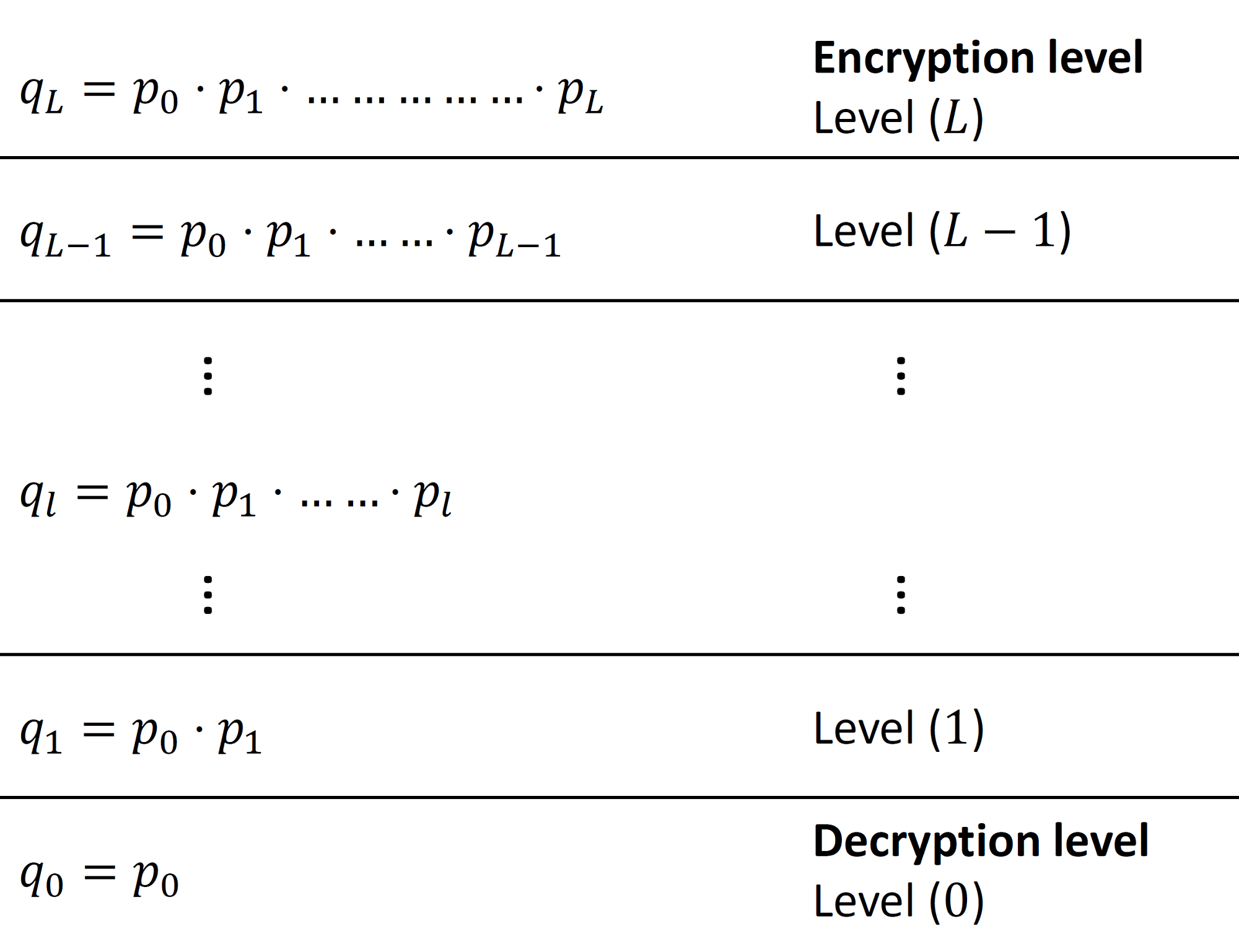
So far we talked about the similarities between BFV and BGV. In the following paragraphs, we describe how the two schemes are different. Firstly, the BFV scheme is typically scale-invariant (or scale-independent), that is, the ciphertext modulus does not change during homomorphic evaluation. On the other hand, BGV is a scale-dependent scheme that defines multiple ciphertext moduli, one modulus per level. As we can see in Figure 1, BGV defines a chain of "small" moduli $\mathcal{Q} = \{ p_0, p_1, \ldots, p_L \}$. Associated with each level $ 0\leq l \leq L$, is a ciphertext big modulus $q_l$. Note that the choice of the small moduli $p_l$'s and consequently the set of big moduli $q_l$'s is not arbitrary and the rationale behind that will become evident later in this article. While performing the homomorphic computation, ciphertexts keep moving from one level to another. The typical flow of ciphertexts is as follows: a freshly encrypted ciphertext starts at level $L$, which we call the encryption level for demonstration. As we compute on the ciphertext, it moves from a higher level $l$ to lower level $l-1$. Eventually and right before decryption, the ciphertext is at level $1$. It should be remarked that the aforementioned downward-restricted flow is the typical flow in the levelled-version of BGV. In $\textit{bootstrappable}$ BGV, the ciphertext can move in both directions (upward or downward) as necessary.

We note that the previous description with fixed levels for encryption and decryption is rather simplified as it is possible to encrypt or decrypt at any level $ 0\leq l \leq L$. It should also be noted that the BFV scheme can also be instantiated as a scale-dependent scheme, which makes this difference between the two schemes controversial.

Figure 1: Scale-dependent BGV ciphertext moduli.

Another less controversial difference between BFV and BGV is the ciphertext structure and how the plaintext message is encrypted. Figure 2 shows the ciphertext structure of BFV and BGV. In the former, the plaintext message is placed towards the Most Significant Bits (MSB) side of the ciphertext coefficient. This is done by scaling the message by the rather large value $\Delta = \lfloor \frac{q}{t} \rfloor$ during encryption. On the other hand, BGV places the message towards the Least Significant Bits (LSB) side of the ciphertext coefficient. It is important that during homomorphic evaluation, the plaintext and noise never overlap so that decryption can recover the expected computation result.

Figure 2: Ciphertext structure in BFV and BGV. MSB stands for most significant bit, $q$ is the ciphertext modulus and $t$ is the plaintext modulus. Adapted from [CKKS17].

In the subsequent sections, we dive deeper into BGV and describe its plaintext and ciphertext spaces, parameters, and the basic cryptographic primitives; key generation, encryption, decryption, homomorphic evaluation, modulus switching and security analysis.

The plaintext and ciphertext spaces of BGV are similar to those in BFV. The plaintext polynomial ring is defined as $\P = R_t = \Z_t[x]/(x^n+1)$, i.e., the set of polynomials with degree less than $n$ and coefficients in $\Z_t$, where the plaintext modulus $t$ and the ring dimension $n$ are both integers. The ciphertext space is defined as $\C = R_{q_l} \times R_{q_l}$, where $R_{q_l} = \Z_{q_l}[x]/(x^n+1)$ and $q_l \in \Z$ is the ciphertext modulus at level $l$. For efficiency purposes, $n$ is usually set as a power-of-2 integer similar to our discussion on BFV. Also, $q$ is usually much greater than $t$ which affects the message expansion rate after encryption. There are security and functionality constraints that should be considered when setting up these parameters. The reader is advised to refer to the homomorphic encryption standard document for a set of recommended parameters [ACC+18].

In addition to the plaintext and ciphertext parameters, BGV defines the following three random distributions:

• $R_2$: mostly used in the encryption keys, is a uniform random distribution used to sample polynomials with integer coefficients in $\{-1,0,1\}$.
• $\mathcal{X}$: is the error distribution defined as a discrete Gaussian distribution with parameters $\mu$ and $\sigma$ over $R$ bounded by some integer $\beta$. According to the current version of the homomorphic encryption standard [ACC+18], $(\mu, \sigma, \beta)$ are set as $(0, \frac{8}{\sqrt{2\pi}}\approx 3.2, \lfloor 6\cdot \sigma \rceil = 19)$.
• $R_q$: is a uniform random distribution over $R_q$ used for sampling polynomials in $\{0,1, \ldots, q-1\}$.

Similar to our discussion in BFV, the input data needs to be encoded to be compatible with the plaintext space $R_t$. We refer the reader to our description of BFV in which we introduced two encoding schemes. They can also be used with BGV without any modification.

The secret key $\textsf{SK}$ is a random ternary polynomial that is generated from $R_2$. The public key $\textsf{PK}$ is a pair of polynomials $(\textsf{PK}_1, \textsf{PK}_2)$ calculated as follows: \begin{align} \textsf{PK}_1 &= [-1(a\cdot \textsf{SK}+t \cdot e)]_{q_L}\\ \textsf{PK}_2 &= a\nonumber \end{align} where $a$ is a random polynomial in $R_{q_l}$, and $e$ is a random error polynomial sampled from $\mathcal{X}$. The notation $[\cdot]_{q_l}$ means that polynomial arithmetic should be done modulo $q_l$. Note how the error is scaled by $t$ here unlike key generation in BFV.

The encryption algorithm takes as input a plaintext message $\textsf{M}$ in $\P$ and the public key $\textsf{PK}$ and outputs ciphertext $\textsf{C}=(\textsf{C}_1,\textsf{C}_2)$ in $\C$ encrypting the input message as a result. Encryption proceeds as follows: we generate three small random polynomials $u$ from $R_2$ and $e_1$ and $e_2$ from $\mathcal{X}$ and compute: \begin{align}\label{eq:encrypt} \textsf{C}_1 &= [\textsf{PK}_1\cdot u + t \cdot e_1 + \textsf{M}]_{q_l}\\ \textsf{C}_2 &= [\textsf{PK}_2\cdot u + t \cdot e_2]_{q_l} \nonumber \end{align} Note how the error polynomial in $\textsf{C}_1$ is scaled by the plaintext modulus $t$. This conforms with what we demonstrated previously in Figure 2 with the message situated in the lower bits of the ciphertext coefficient while the noise can grow in the upper bits.

The decryption procedure reverses encryption by taking as input the ciphertext and the secret key $\textsf{SK}$. It outputs the plaintext message $\textsf{M}$ given that the noise did not grow out of control during computation. Decryption proceeds as follows: \begin{equation} \label{eq:decryption} \textsf{M} = \big[ [\textsf{C}_1+\textsf{C}_2\cdot \textsf{SK}]_{q_l} \big]_t \end{equation} In order to check why decryption works and under which conditions, let us expand Equation \eqref{eq:decryption} as follows assuming that decryption occurs right after encryption for simplicity of exposition: \begin{align} \label{eq:dec:proof} \textsf{C}_1+\textsf{C}_2\cdot\textsf{SK} &= \textsf{PK}_1 \cdot u + t \cdot e_1 + \textsf{M} + (\textsf{PK}_2\cdot u + t \cdot e_2)\cdot \textsf{SK}\\ &= -(a\cdot \textsf{SK}+t \cdot e)\cdot u + t \cdot e_1+ \textsf{M} + a\cdot u \cdot \textsf{SK} + t \cdot e_2\cdot \textsf{SK} \nonumber\\ &= \cancel{-a\cdot u \cdot \textsf{SK}} - t \cdot e\cdot u+t\cdot e_1+ \textsf{M} + \cancel{a\cdot u \cdot \textsf{SK}} + t \cdot e_2\cdot \textsf{SK} \nonumber\\ &= \textsf{M} - t \cdot e\cdot u + t \cdot e_1 + t \cdot e_2\cdot\textsf{SK} \nonumber\\ &= \textsf{M} + t\cdot v \nonumber \end{align} By reducing the result above modulo $t$, we get rid of the noise vector $v$ and recover $\textsf{M}$ without the noise. But there is a caveat here that is related to the norm of $v$. Decryption works as long as ${\left\| v \right\|}_\infty < \dfrac{q_l}{2t}$, where ${\left\| v \right\|}_\infty$ is defined as the largest absolute coefficient in $v$. The bound is set so that the magnitude of the noise does not grow too much and destroy the message.

What differentiates FHE from classic encryption schemes are the homomorphic evaluation procedures. Here we study the two main homomorphic operations: addition and multiplication.
As shown in Equation \eqref{eq:homo:add}, homomorphic addition takes as input two ciphertexts $\textsf{C}^{(1)}$ and $\textsf{C}^{(2)}$ defined with respect to the same modulus $q_l$ and returns a ciphertext ($\textsf{C}_3$) that contains an encryption of the summation of the two plaintext messages encrypted in the input, that is, $\textsf{Decryption}(\textsf{C}_3, \textsf{SK}) = \textsf{M}_1 + \textsf{M}_2 \mod t$. This will apply as long as the error in the addend ciphertexts is not too large. In order to understand this, let us analyze the homomorphic addition procedure. Equation \eqref{eq:homo:add} is fairly simple, we just add the corresponding polynomials in each ciphertext. \begin{equation}\label{eq:homo:add} \textsf{EvalAdd}(\textsf{C}^{(1)}, \textsf{C}^{(2)}) = ([\textsf{C}^{(1)}_1 + \textsf{C}^{(2)}_1]_{q_l}, [\textsf{C}^{(1)}_2 + \textsf{C}^{(2)}_2]_{q_l}) = ( \textsf{C}^{(3)}_1, \textsf{C}^{(3)}_2) = \textsf{C}^{(3)} \end{equation} In order to see why this works, let us break Equation \eqref{eq:homo:add} as follows: assume that $\textsf{C}^{(1)}$ and $\textsf{C}^{(2)}$ are fresh encryptions of $\textsf{M}^{(1)}$ and $\textsf{M}^{(2)}$. Algebraically, they can be expressed as follows (See Equation \eqref{eq:encrypt}): \begin{align} \label{eq:homo:add_det1} \textsf{C}^{(1)} &= ([\textsf{PK}_1\cdot u^{(1)} + t\cdot e_1^{(1)} + \textsf{M}^{(1)}]_{q_l}, [\textsf{PK}_2 \cdot u^{(1)} + t \cdot e_2^{(1)}]_{q_l})\\ \textsf{C}^{(2)} &= ([\textsf{PK}_1\cdot u^{(2)} + t\cdot e_1^{(2)} + \textsf{M}^{(2)}]_{q_l}, [\textsf{PK}_2 \cdot u^{(2)} + t\cdot e_2^{(2)}]_{q_l}) \nonumber \end{align} By substituting $\textsf{C}^{(1)}$ and $\textsf{C}^{(2)}$ in Equation \eqref{eq:homo:add} we get the following: \begin{align} \textsf{C}^{(3)} &= ( \textsf{C}^{(3)}_1, \textsf{C}^{(3)}_2)\\ ={}& ( [\textsf{PK}_1\cdot(u^{(1)}+u^{(2)})+t(e_1^{(1)}+e_1^{(2)})+ (\textsf{M}^{(1)}+\textsf{M}^{(2)})]_{q_l}, \nonumber \\ {}&~[\textsf{PK}_2\cdot(u^{(1)}+u^{(2)})+t(e_2^{(1)}+e_2^{(2)})]_{q_l} ) \nonumber \\ ={}& ( [\textsf{PK}_1\cdot u^{(3)}+t\cdot e_1^{(3)}+ (\textsf{M}^{(1)}+\textsf{M}^{(2)})]_{q_l}, [\textsf{PK}_2 \cdot u^{(3)}+t\cdot e_2^{(3)}]_{q_l} )\label{eq:homo:add_det2} \end{align} It is straightforward to see that Equation \eqref{eq:homo:add_det2} has the form of a valid ciphertext encrypting $\textsf{M}^{(3)} = \textsf{M}^{(1)} + \textsf{M}^{(2)}$. Note that the error term in $\textsf{C}^{(3)}$ is approximately, following a worst-case scenario analysis, the sum of the noise terms in the input ciphertexts, i.e., the noise grows additively.
Homomorphic multiplication takes as input two ciphertexts $\textsf{C}^{(1)}$ and $\textsf{C}^{(2)}$ defined with respect to the same modulus $q_l$ and returns a ciphertext ($\textsf{C}_3$) that contains an encryption of the product of the two plaintext messages encrypted in the input ciphertexts, that is, $\textsf{Decryption}(\textsf{C}_3, \textsf{SK}) = \textsf{M}_1 \cdot \textsf{M}_2 \mod t$.

In the following analysis, we interpret the decryption formula as a ciphertext evaluation at $\textsf{SK}$: \begin{align} \textsf{C}^{(1)}(\textsf{SK}) &= \textsf{M}^{(1)}+t \cdot v_1+ q_l \cdot r_1\\ \textsf{C}^{(2)}(\textsf{SK}) &= \textsf{M}^{(2)}+t \cdot v_2+q_l \cdot r_2 \nonumber \end{align} Multiplying the ciphertexts gives us: \begin{equation}\label{eq:homo:mul} \begin{split} (\textsf{C}^{(1)} \cdot \textsf{C}^{(2)})(\textsf{SK}) =& \textsf{M}^{(1)}\cdot \textsf{M}^{(2)} + t(\textsf{M}^{(1)}\cdot v_2+\textsf{M}^{(2)}\cdot v_1)+\\ &q_l\cdot t (v_1\cdot r_2 + v_2\cdot r_1) + q_l\cdot (\textsf{M}^{(1)}\cdot r_2 + \textsf{M}^{(2)} \cdot r_1)+\\ &t^2\cdot v_1 \cdot v_2 + q{_l}^2 \cdot r_1 \cdot r_2\\ =& \textsf{M}^{(1)}\cdot \textsf{M}^{(2)} + t(\textsf{M}^{(1)}\cdot v_2+\textsf{M}^{(2)}\cdot v_1 + t\cdot v_1 \cdot v_2) \end{split} \end{equation} The decryption formula of the product ciphertext has the structure of a valid ciphertext encrypting ($\textsf{M}^{(1)}\cdot \textsf{M}^{(2)}$) with noise $v = \textsf{M}^{(1)}\cdot v_2+\textsf{M}^{(2)}\cdot v_1 + t\cdot v_1 \cdot v_2$. Note how the noise term grows multiplicatively as the product of the noise in the input ciphertexts (the term $t\cdot v_1 \cdot v_2$). This means that as we go deeper in the computation, the noise grows exponentially. To resolve this problem, BGV uses $\textsf{ModSwitch}$ to reduce the rate at which multiplication noise grows. $\textsf{ModSwitch}$ will be described later on in this article.

From the above discussion, we can deduce that $\textsf{EvalMult}$ can be evaluated as polynomial multiplication of the input ciphertexts as can be shown in the following equation: \begin{equation} \begin{split} \textsf{EvalMult}(\textsf{C}^{(1)}, \textsf{C}^{(2)}) = (& [ \textsf{C}^{(1)}_1\cdot\textsf{C}^{(2)}_1 ]_{q_l}, [ \textsf{C}^{(1)}_1 \cdot \textsf{C}^{(2)}_2 + \textsf{C}^{(1)}_2 \cdot \textsf{C}^{(2)}_1 ]_{q_l}, \\& [ \textsf{C}^{(1)}_2 \cdot \textsf{C}^{(2)}_2 ]_{q_l} ) \end{split} \end{equation} $\textsf{EvalMult}$ increases the number of ring elements in the resulting ciphertext from 2 to 3. Moreover, the product ciphertext is defined with respect to $\textsf{SK}^2$ rather than the original $\textsf{SK}$, that is, it is decryptable using $\textsf{SK}^2$. In order to reduce the number of elements back to 2 and make the ciphertext decryptable using $\textsf{SK}$, the $\textsf{Relinearization}$ procedure, described next, can be used.

This procedure is used to overcome the two issues that arise in $\textsf{EvalMult}$, ciphertext expansion and defining the ciphertext with respect to the original $\textsf{SK}$. We described this procedure thoroughly in our BFV article in Section 9 ($\textsf{Relinearization}$). We reiterate briefly here due to some minor changes related to the ciphertext modulus.

The problem we are trying to solve can be formulated as follows: let $\textsf{C}^{*} = \{\textsf{C}^{*}_1, \textsf{C}^{*}_2, \textsf{C}^{*}_3\}$. Our goal is to find $\hat{\textsf{C}}^{*} = \{\hat{\textsf{C}}^{*}_1, \hat{\textsf{C}}^{*}_2\}$ such that: \begin{equation} [\textsf{C}^{*}_1 + \textsf{C}^{*}_2\cdot \textsf{SK} + \textsf{C}^{*}_3 \cdot \textsf{SK}^2]_{q_l} \approx [\hat{\textsf{C}}^{*}_1 + \hat{\textsf{C}}^{*}_2 \cdot \textsf{SK} + r]_{q_l} \end{equation}

Access to $\textsf{SK}^2$ is provided by means of the evaluation key $\textsf{EK} = (-(a\cdot \textsf{SK} + e) + \textsf{SK}^2, a)$. Note that this is a masked version of $\textsf{SK}^2$ since $\textsf{EK}_1 + \textsf{EK}_2 \cdot \textsf{SK} = \textsf{SK}^2 - e$. Now we can compute $\hat{\textsf{C}^{*}}$ as follows: \begin{align}\label{eq:relin} \hat{\textsf{C}}^{*}_1 &= [\textsf{C}^*_1 + \textsf{EK}_1\cdot \textsf{C}^*_3]_{q_l}\\ \hat{\textsf{C}}^{*}_2 &= [\textsf{C}^*_2 + \textsf{EK}_2\cdot \textsf{C}^*_3]_{q_l} \nonumber \end{align}

If we write the decryption formula for Equation \eqref{eq:relin} we obtain what we want as follows: \begin{align} \hat{\textsf{C}}^{*}_1 + \hat{\textsf{C}}^{*}_2 \cdot \textsf{SK} &= \textsf{C}^*_1 + \textsf{EK}_1\cdot \textsf{C}^*_3 + \textsf{SK}\cdot (\textsf{C}^*_2 + \textsf{EK}_2\cdot \textsf{C}^*_3)\\ &= \textsf{C}^*_1 + \textsf{C}^*_2 \cdot \textsf{SK} + \textsf{C}^*_3\cdot(\textsf{EK}_1 + \textsf{EK2} \cdot \textsf{SK} )\nonumber\\ &= \textsf{C}^*_1 + \textsf{C}^*_2 \cdot \textsf{SK} + \textsf{C}^*_3 \cdot \textsf{SK}^2 + \textsf{C}^*_3 \cdot e \nonumber \end{align}

As mentioned previously, $\textsf{ModSwitch}$ is used to control the multiplication noise. This notion was first introduced in [BGV14], and it exploits the fact that given a ciphertext $\textsf{C}$ defined with respect to modulus $q$ and secret key $\textsf{SK}$, it can be transformed into an equivalent ciphertext $\textsf{C}'$ defined with respect to another modulus $q'$ and the same secret key $\textsf{SK}$ such that: \begin{equation} [\textsf{C}(\textsf{SK})]_q = [\textsf{C}'(\textsf{SK})]_{q'} \end{equation}

The transformation is done by scaling the coefficients of $\textsf{C}$ by the quantity $q'/q$ and some suitable rounding. To reduce the noise magnitude, we choose a fairly smaller $q'$ than $q$, which allows us to scale down the multiplication noise.

Note that in the BGV context, $q$ can be at any level $l$, i.e., $q_l$; and $q'$ in this context is simply $q_{l-1}$. Moreover, the ciphertext moduli $q_l,~\forall~0\leq l \leq L$ are chosen such that they are equivalent modulo $t$. This results in scaling down the noise without affecting the encrypted plaintext message. It is as if we are scaling by 1 from the plaintext perspective.

$\textsf{ModSwitch}$ can be computed as shown in Equation \eqref{eq:mod:switch}, where $[\cdot]$ is a suitable rounding function. The transformed ciphertext $\textsf{C}'$ is defined with respect to the new modulus $q'$. \begin{equation}\label{eq:mod:switch} \textsf{C}' = \big[ \dfrac{q'}{q} \cdot \textsf{C} \big] \end{equation}

To the best of our knowledge, BGV is still considered a secure scheme with no known attacks published in the literature. Its security stems from the hardness of the RLWE problem. We remark that choosing optimal BGV parameters that maximize performance and respect both security and functionality constraints is a fairly complex task and it is best to consult expert cryptographers to do so. For a brief security analysis and a set of recommended parameters for BGV (and other FHE schemes), we refer the reader to the homomorphic encryption standard [ACC+18].

[ACC+18] Martin Albrecht, Melissa Chase, Hao Chen, Jintai Ding, Shafi Goldwasser, Sergey Gorbunov, Shai Halevi, Jeffrey Hoffstein, Kim Laine, Kristin Lauter, Satya Lokam, Daniele Micciancio, Dustin Moody, Travis Morrison, Amit Sahai, and Vinod Vaikuntanathan. Homomorphic encryption security standard. Technical report, HomomorphicEncryption. org, Toronto, Canada, November 2018.

[BGV14] Zvika Brakerski, Craig Gentry, and Vinod Vaikuntanathan. (leveled) fully homomorphic encryption without bootstrapping. ACM Transactions on Computation Theory (TOCT), 6(3):1–36, 2014.

[Bra12] Zvika Brakerski. Fully homomorphic encryption without modulus switching from classical gapsvp. In Annual Cryptology Conference, pages 868–886. Springer, 2012.

[CKKS17] Jung Hee Cheon, Andrey Kim, Miran Kim, and Yongsoo Song. Homomorphic encryption for arithmetic of approximate numbers. In International Conference on the Theory and Application of Cryptology and Information Security, pages 409–437. Springer, 2017.

[ElG21] ElGamal Encryption. Elgamal encryption — Wikipedia, the free encyclopedia, 2021. [Online; accessed 2021-June-2021].

[FV12] Junfeng Fan and Frederik Vercauteren. Somewhat practical fully homomorphic encryption. 2012. https://eprint.iacr.org/2012/144.

[LPR13] Vadim Lyubashevsky, Chris Peikert, and Oded Regev. On ideal lattices and learning with errors over rings. Journal of the ACM (JACM), 60(6):1–35, 2013.